Fitting two-dimensional data
nDspec allows users to fit generic two-dimensional data, using identical methods, optimizers, inference etc as the other fitters in the package. This method allows great freedom for users, as in principle they can fit any dataset they can import provided they have a model for it.
If users wish for one of the two dimensions to be photon energy, then they can provide an instrument response matrix, and the fitter will automatically fold the two-dimensional model through the response when evaluating the likelihood.
[1]:
import numpy as np
import warnings
import os
import sys

import matplotlib.pyplot as plt
from matplotlib import rc, rcParams
rc('text',usetex=True)
rc('font',**{'family':'serif','serif':['Computer Modern']})
plt.rcParams.update({'font.size': 17})

from lmfit import Model as LM_Model
from lmfit import Parameters as LM_Parameters

sys.path.append('/home/matteo/Software/nDspec/src/')
from ndspec.Response import ResponseMatrix
from ndspec.FitTwoD import FitTwoD
import ndspec.Models as models
Dynamical power spectra
As a first example, let us fit a power spectrum where a broad component remains constant, but with the addition of a QPO whose centroid varies over some phase. We will begin by defining a model and two grids to generate fake data from:
[2]:
#lorentzian model with one narrow lorentzian drifting over phase
def lorentz(freq,peak_f,q,rms):
    par_array = np.array([peak_f,q,rms])
    model = models.lorentz(freq,par_array)
    return model

def sin_wave(phase,norm,center):
    return norm*np.sin(phase*2*np.pi)+center

#x_grid is phase, y_grid is frequency
def twod_lorentzians(x_axis,y_axis,peak_1,peak_2,q_1,q_2,rms_1,rms_2,mod_norm):
    peak_2_mod = sin_wave(x_axis,mod_norm,peak_2)
    model = np.zeros((len(x_axis),len(y_axis)))
    for i, peak in enumerate(peak_2_mod):
        model[i,:] = lorentz(y_axis,peak,q_2,rms_2)*y_axis
    model = model + (lorentz(y_axis,peak_1,q_1,rms_1)*y_axis).reshape(1,(len(y_axis)))
    return model.T

#define our grid of
phase_grid = np.linspace(0,1,30)
freq_grid = np.geomspace(1e-1,10,50)
We can now take our model, and draw random numbers from it distributed along a Gaussian function to generate our data, using a standard deviation of 5% to fake the errors. Note that the shape of these arrays is (50x30) - 30 rows in phase, and 50 columns in Fourier frequency:
[3]:
peak_1 = 1
q_1 = 1e-1
rms_1 = 2e-2
peak_2 = 5
q_2 = 5
rms_2 = 1e-2
#this controls the modulation of the centroid frequency of the QPO
mod_norm = 2.
starting_model = twod_lorentzians(phase_grid,freq_grid,peak_1,peak_2,q_1,q_2,rms_1,rms_2,mod_norm)
dynamical_psd = np.random.normal(loc=starting_model,scale=0.05*starting_model,size=starting_model.shape)
dynamical_psd_err = 0.05*dynamical_psd
print(dynamical_psd.shape,dynamical_psd_err.shape)
#test plot in 1d with errors
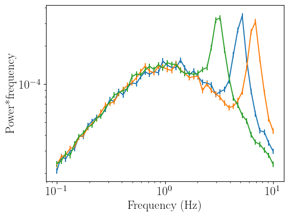
fig, ax1 = plt.subplots(1,1,figsize=(6.,4.5))
ax1.errorbar(freq_grid,dynamical_psd[:,0],yerr=dynamical_psd_err[:,0])
ax1.errorbar(freq_grid,dynamical_psd[:,10],yerr=dynamical_psd_err[:,10])
ax1.errorbar(freq_grid,dynamical_psd[:,20],yerr=dynamical_psd_err[:,20])
ax1.set_xscale("log")
ax1.set_yscale("log")
ax1.set_xlabel("Frequency (Hz)")
ax1.set_ylabel("Power*frequency")
#test plot in 2d
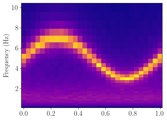
fig, ax2 = plt.subplots(1,1,figsize=(6.,4.5))
ax2.pcolormesh(phase_grid,freq_grid,dynamical_psd,cmap="plasma",shading='auto',linewidth=0)
ax2.set_ylabel("Phase")
ax2.set_ylabel("Frequency (Hz)")
(50, 30) (50, 30)
[3]:
Text(0, 0.5, 'Frequency (Hz)')
Now that we have generated our fake data, we can initialize a FitTWoD object and use the set_data method to assign the data, error, as well as the grids along the X (column_grid) and Y (row_grid) axis over which the data is defined.
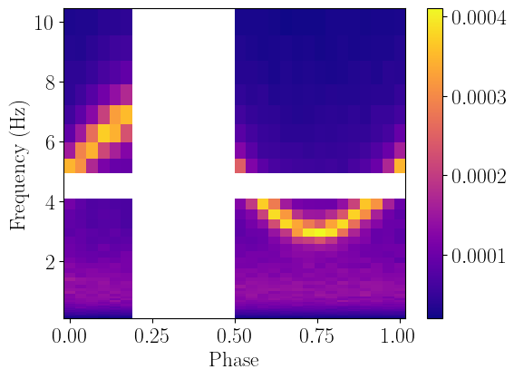
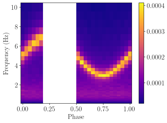
We can then plot the data using the plot_data method to make sure everything worked out correctly. If at any point during our work we wish to ignore (or stop ignoring) any data bins, we can do so with the ignore_row, notice_row, ignore_column, or notice_column methods:
[4]:
dynamical_psd_fit = FitTwoD()
dynamical_psd_fit.set_data(dynamical_psd,dynamical_psd_err,column_grid=phase_grid,row_grid=freq_grid)
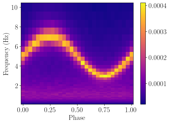
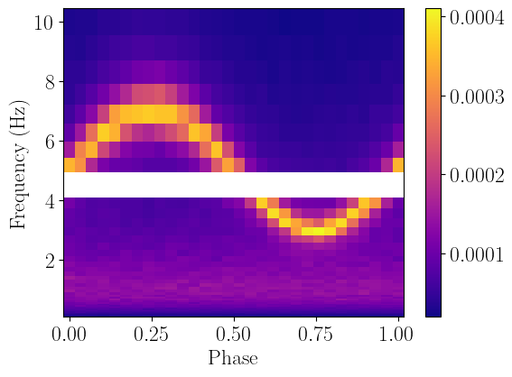
dynamical_psd_fit.plot_data(x_name="Phase",y_name="Frequency (Hz)")
dynamical_psd_fit.ignore_rows(4,5)
dynamical_psd_fit.plot_data(x_name="Phase",y_name="Frequency (Hz)")
dynamical_psd_fit.ignore_columns(0.2,0.5)
dynamical_psd_fit.plot_data(x_name="Phase",y_name="Frequency (Hz)")
dynamical_psd_fit.notice_rows(4,5)
dynamical_psd_fit.plot_data(x_name="Phase",y_name="Frequency (Hz)")
dynamical_psd_fit.notice_columns(0.2,0.5)
dynamical_psd_fit.plot_data(x_name="Phase",y_name="Frequency (Hz)")

We can now define a model to fit our data - conveniently, we will re-use the same function we used to fake the data in the first place.
When defining multi-dimensional models like this, we have to be extremely careful to ensure the rows and columns actually end up in the right bins. In this case, we need to transpose the output of the two_lorentzians model function in order to be compatible with the data - this is due to a quirk of how numpy flattens the arrays once they are imported in the fitter.
We also need to make sure to specify that in our model, the independent variables are x_axis and y_axis, which need to be in the model definition in order for the fitter object to use the appropriate grids.
Once we have set up our model and parameters, we can quickly compare the model and data with the plot_model method:
[5]:
#the transpose here and above are necessary to avoid mixing rows and columns
def twod_lorentzians_eval(x_axis,y_axis,peak_1,peak_2,q_1,q_2,rms_1,rms_2,mod_norm):
    model = twod_lorentzians(x_axis,y_axis,peak_1,peak_2,q_1,q_2,rms_1,rms_2,mod_norm)
    model = model.T
    return model

two_lorentzians = LM_Model(twod_lorentzians_eval,independent_vars=['x_axis','y_axis'])
dynamical_psd_fit.set_model(two_lorentzians)

start_params = two_lorentzians.make_params(peak_1=dict(value=2,min=0,max=10),
                                           peak_2=dict(value=5,min=0,max=10),
                                           q_1=dict(value=0.1,min=0,max=1),
                                           q_2=dict(value=3,min=1,max=10),
                                           rms_1=dict(value=0.1,min=0,max=1),
                                           rms_2=dict(value=0.1,min=0,max=1),
                                           mod_norm=dict(value=1,min=0,max=3),
                                           )
dynamical_psd_fit.set_params(start_params)
dynamical_psd_fit.model_params.pretty_print()
dynamical_psd_fit.plot_model(x_name="Phase",y_name="Frequency (Hz)")
 - Adding parameter "peak_1"
 - Adding parameter "peak_2"
 - Adding parameter "q_1"
 - Adding parameter "q_2"
 - Adding parameter "rms_1"
 - Adding parameter "rms_2"
 - Adding parameter "mod_norm"
Name         Value      Min      Max   Stderr     Vary     Expr Brute_Step
mod_norm         1        0        3     None     True     None     None
peak_1           2        0       10     None     True     None     None
peak_2           5        0       10     None     True     None     None
q_1            0.1        0        1     None     True     None     None
q_2              3        1       10     None     True     None     None
rms_1          0.1        0        1     None     True     None     None
rms_2          0.1        0        1     None     True     None     None
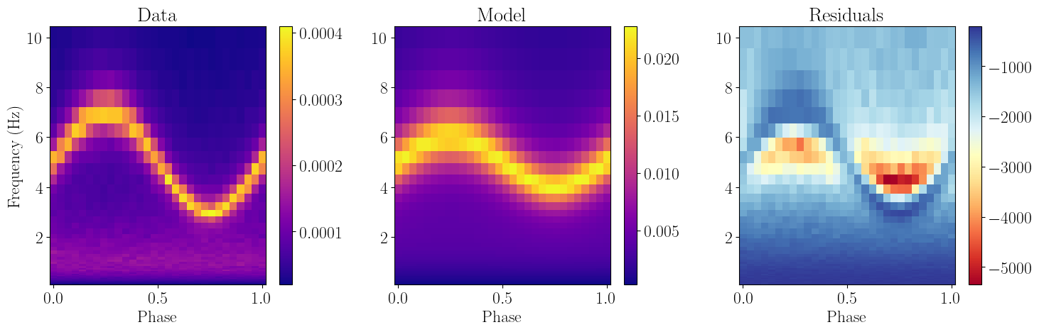
Now that our data and model are defined, we can simply optimize the likelihood function (which by definition is the chi squared statistic, but can be set to any likelihood the user wants, as is the case for all other fitters) and re-plot the model against the data:
[6]:
dynamical_psd_fit.fit_data()
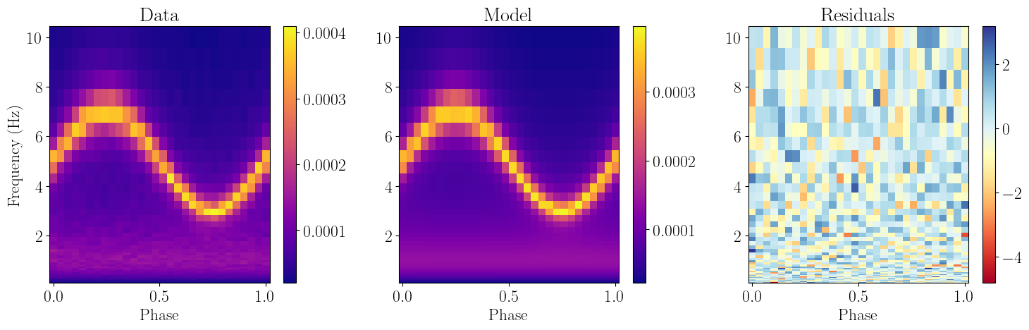
dynamical_psd_fit.plot_model(x_name="Phase",y_name="Frequency (Hz)")
-----------------------
[[Fit Statistics]]
    # fitting method   = leastsq
    # function evals   = 81
    # data points      = 1500
    # variables        = 7
    fit statistic      = 1500.1869632947391
    reduced statistic  = 1.0048137731378024
    Akaike info crit   = 14.186951643949245
    Bayesian info crit = 51.37949435358135
[[Parameters]]
    peak_1:    0.99788167 +/- 0.00236874 (0.24%) (init = 2), model_value = 0.9978817
    peak_2:    5.00050288 +/- 0.00327420 (0.07%) (init = 5), model_value = 5.000503
    q_1:       0.10097227 +/- 0.00244989 (2.43%) (init = 0.1), model_value = 0.1009723
    q_2:       4.94913322 +/- 0.04376318 (0.88%) (init = 3), model_value = 4.949133
    rms_1:     0.01993095 +/- 1.7319e-05 (0.09%) (init = 0.1), model_value = 0.01993095
    rms_2:     0.00998931 +/- 2.8485e-05 (0.29%) (init = 0.1), model_value = 0.009989306
    mod_norm:  2.00842015 +/- 0.00449490 (0.22%) (init = 1), model_value = 2.00842
Time-resolved spectroscopy
Having an energy-dependent model is the same, except we need to use a response matrix. In this case, we will simulate and fit a pulse profile, using a black body with a constant temperature, and a normalization which varies over a phase.
First, we begin by loading in the NICER response matrix, and rebinning it to down to 40 channels (for which we need to specify 41 channel edges, which we do in rebin_bonds):
[7]:
#now do the same but with energy dependent stuff

rmfpath = os.getcwd()+"/data/nicer-rmf6s-teamonly-array50.rmf"
nicer_matrix = ResponseMatrix(rmfpath)
arfpath = os.getcwd()+"/data/nicer-consim135p-teamonly-array50.arf"
nicer_matrix.load_arf(arfpath)

rebin_bounds = np.geomspace(0.5,10,41)
rebin_bounds = np.append(np.min(nicer_matrix.emin),rebin_bounds)
rebin_bounds = np.append(rebin_bounds,np.max(nicer_matrix.emax))
rebin_bounds_lo = rebin_bounds[:-1]
rebin_bounds_hi = rebin_bounds[1:]
rebin_response = nicer_matrix.rebin_channels(rebin_bounds_lo,rebin_bounds_hi)
Arf missing, please load it
Arf loaded
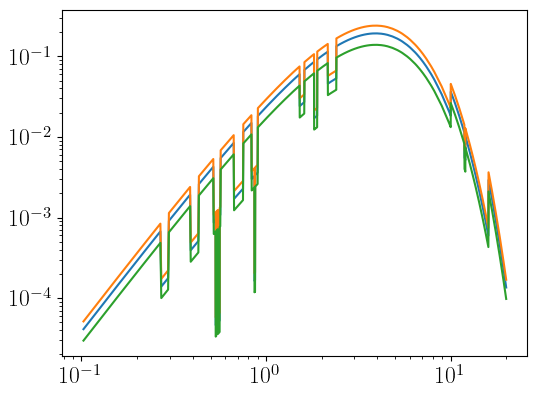
As before, we need to simulate the data. Note that it is common for energy-dependent models to provide fluxes in units integrated over each bit, so we have to do the same for our dataset as well. As before, the size of our model is numer of rows times number of columns - so here, that is 3451 energy bins (from the NICER response) times 30 phase bins
[8]:
def pulsing_bb(ear,x_axis,norm_bb,kT,norm_mod):
var_norm = sin_wave(x_axis,norm_mod,norm_bb)
energ = 0.5*(ear[1:]+ear[:-1])
model = np.zeros((len(x_axis),len(energ)))
for i, phasenorm in enumerate(var_norm):
bb_array = np.array([phasenorm,kT])
#the np.diff(ear) is the bin width, so we are effectively integrating
#over each energy bin here
model[i,:] = models.bbody(energ,bb_array)*np.diff(ear)
model = model.T
return model
ear_bins = np.append(nicer_matrix.energ_lo,nicer_matrix.energ_hi[-1])
energ_bins = 0.5*(nicer_matrix.energ_lo+nicer_matrix.energ_hi)
const_norm = 1
ktbb = 1
modulation = 0.3
model_varbb = pulsing_bb(ear_bins,phase_grid,const_norm,ktbb,modulation)
print(model_varbb.shape)
#test plot in 1d with errors
fig, ax1 = plt.subplots(1,1,figsize=(6.,4.5))
ax1.errorbar(energ_bins,model_varbb[:,0]*energ_bins**2)
ax1.errorbar(energ_bins,model_varbb[:,10]*energ_bins**2)
ax1.errorbar(energ_bins,model_varbb[:,20]*energ_bins**2)
ax1.set_xscale("log")
ax1.set_yscale("log")
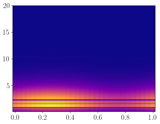
#test plot in 2d
renorm_bins = np.diff(ear_bins).reshape((len(energ_bins),1))
fig, ax2 = plt.subplots(1,1,figsize=(6.,4.5))
ax2.pcolormesh(phase_grid,energ_bins,model_varbb,cmap="plasma",shading='auto',linewidth=0)
(3451, 30)
[8]:
<matplotlib.collections.QuadMesh at 0x7bba06af1ae0>
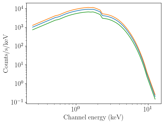
We are now going to fold our model through the rebinned response, which will leave us with 42 channels times 30 phase bins. Note that we always have to add two channels to the binning we chose at the start: from the very start of the response to the start first bin we specify, and from the last bin we specify to the end of the response. This is necessary in order for the folding to be calculated correctly, and is taken care of automatically in nDspec.
[9]:
#now to simulate data
rebin_chans = 0.5*(rebin_bounds_lo+rebin_bounds_hi)
folded_varbb = rebin_response.convolve_response(model_varbb)
print(folded_varbb.shape)
#test plot in 1d with errors
fig, ax1 = plt.subplots(1,1,figsize=(6.,4.5))
ax1.errorbar(rebin_chans,folded_varbb[:,0])
ax1.errorbar(rebin_chans,folded_varbb[:,10])
ax1.errorbar(rebin_chans,folded_varbb[:,20])
ax1.set_xscale("log")
ax1.set_yscale("log")
ax1.set_xlabel("Channel energy (keV)")
ax1.set_ylabel("Counts/s/keV")
#test plot in 2d
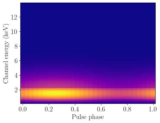
fig, ax2 = plt.subplots(1,1,figsize=(6.,4.5))
ax2.pcolormesh(phase_grid,rebin_chans,folded_varbb,cmap="plasma",shading='auto',linewidth=0)
ax2.set_xlabel("Pulse phase")
ax2.set_ylabel("Channel energy (keV)")
(42, 30)
[9]:
Text(0, 0.5, 'Channel energy (keV)')
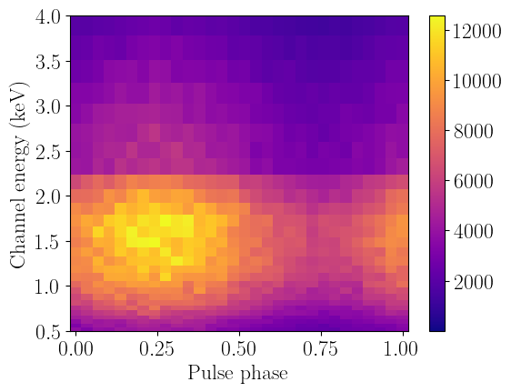
Now that we folded the model through the response, we can generate fake data from it again. Once again we will use a Gaussian errors with a 5% standard deviation for simplicity, although technically in this case we should be using a Poisson distribution since we are simulating photon counts.
[10]:
renorm_ewidths = (rebin_response.emax-rebin_response.emin).reshape((rebin_response.n_chans,1))

simulate_pulse = np.random.normal(loc=folded_varbb,scale=0.05*folded_varbb,size=folded_varbb.shape)
simulate_pulse_err = 0.05*simulate_pulse

#test plot in 2d
fig, ax2 = plt.subplots(1,1,figsize=(6.,4.5))
data_plot = ax2.pcolormesh(phase_grid,rebin_chans,simulate_pulse,cmap="plasma",shading='auto',linewidth=0)
fig.colorbar(data_plot, ax=ax2)
ax2.set_xlabel("Pulse phase")
ax2.set_ylabel("Channel energy (keV)")
ax2.set_ylim([0.5,4])
[10]:
(0.5, 4.0)
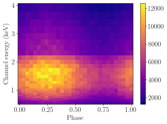
Now we can load the data and ignore the bins (with low signal) below 0.5 and above 4 keV:
[11]:
fit_phase = FitTwoD()
fit_phase.set_data(simulate_pulse,simulate_pulse_err,column_grid=phase_grid,row_grid=rebin_bounds,response=nicer_matrix)
fit_phase.ignore_rows(0,0.5)
fit_phase.ignore_rows(4,20)
fit_phase.plot_data(x_name="Phase",y_name="Channel energy (keV)")
Finally, we will define a model identically to before and then fit the data. Not that the independent variable names are identical, and that we do not need to include folding the instrument response in our model definition, as that is now done automatically when evaluating the model now:
[12]:
def pulsing_bb_eval(y_axis,x_axis,norm_bb,kT,norm_mod):
    model = pulsing_bb(y_axis,x_axis,norm_bb,kT,norm_mod)
    model = model.T
    return model

pulse_model = LM_Model(pulsing_bb_eval,independent_vars=['y_axis','x_axis'])
fit_phase.set_model(pulse_model)

start_params = pulse_model.make_params(norm_bb=dict(value=1,min=0,max=10),
                                       kT=dict(value=2,min=0,max=10),
                                       norm_mod=dict(value=0.2,min=0,max=1),
                                       )
fit_phase.set_params(start_params)
fit_phase.model_params.pretty_print()
fit_phase.plot_model(x_name="Phase",y_name="Channel energy (keV)")
 - Adding parameter "norm_bb"
 - Adding parameter "kT"
 - Adding parameter "norm_mod"
Name         Value      Min      Max   Stderr     Vary     Expr Brute_Step
kT               2        0       10     None     True     None     None
norm_bb          1        0       10     None     True     None     None
norm_mod       0.2        0        1     None     True     None     None
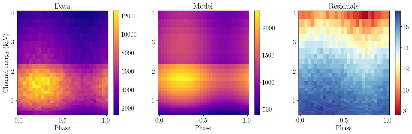
[13]:
fit_phase.fit_data()
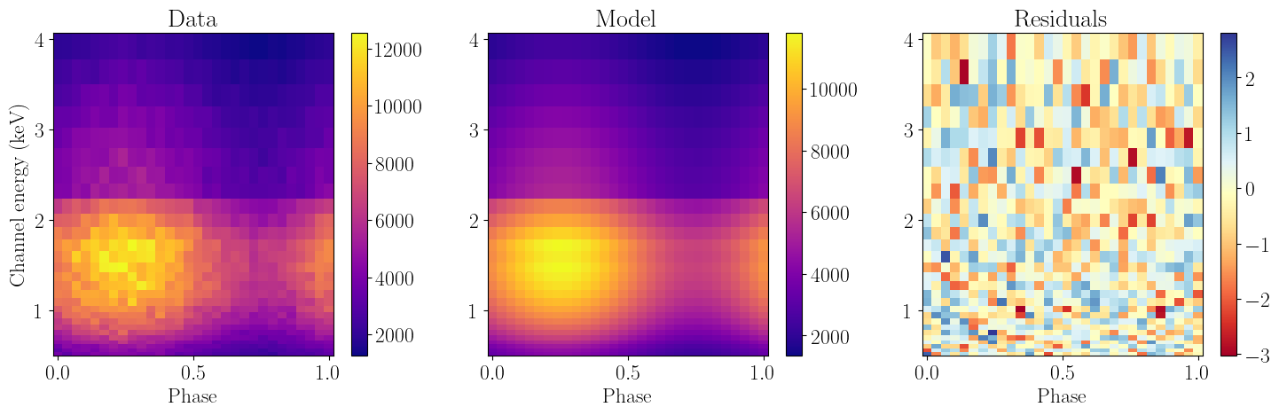
fit_phase.plot_model(x_name="Phase",y_name="Channel energy (keV)")
-----------------------
[[Fit Statistics]]
    # fitting method   = leastsq
    # function evals   = 29
    # data points      = 840
    # variables        = 3
    fit statistic      = 834.4022107305332
    reduced statistic  = 0.996896309116527
    Akaike info crit   = 0.3834755180334355
    Bayesian info crit = 14.583681193545512
[[Parameters]]
    norm_bb:   0.99531422 +/- 0.00180968 (0.18%) (init = 1), model_value = 0.9953142
    kT:        0.99986791 +/- 6.8388e-04 (0.07%) (init = 2), model_value = 0.9998679
    norm_mod:  0.29535150 +/- 0.00267648 (0.91%) (init = 0.2), model_value = 0.2953515