Simulating Observations

nDspec allows users to simulate three spectral-timing products for proposals, checking results, etc: lightcurves, time-averaged spectra, and lag energy spectra, starting from user-defined models and observation details.

import sys
import os
import gc
import numpy as np
import matplotlib.pyplot as plt

from lmfit import Model as LM_Model
from lmfit import Parameters as LM_Parameters

sys.path.append(os.path.dirname(os.path.dirname(os.path.abspath('__file__'))))

from ndspec.Response import ResponseMatrix
from ndspec.Timing import PowerSpectrum, CrossSpectrum
import ndspec.Models as models

How to simulate a lightcurve

Simulating a lightcurve from an assumed model power spectrum is extremely simple, and relies on the implementation of the Timmer and Konig algorithm in Stingray. We begin by defining a model power spectrum, starting from a time grid which will inform the Fourier frequencies our model will probe:

#Define our time grid and power spectrum object
obs_time = 5e2
dt = 0.05
N = int(obs_time/dt)
times = np.linspace(dt,obs_time,N)

psd_model = PowerSpectrum(times)

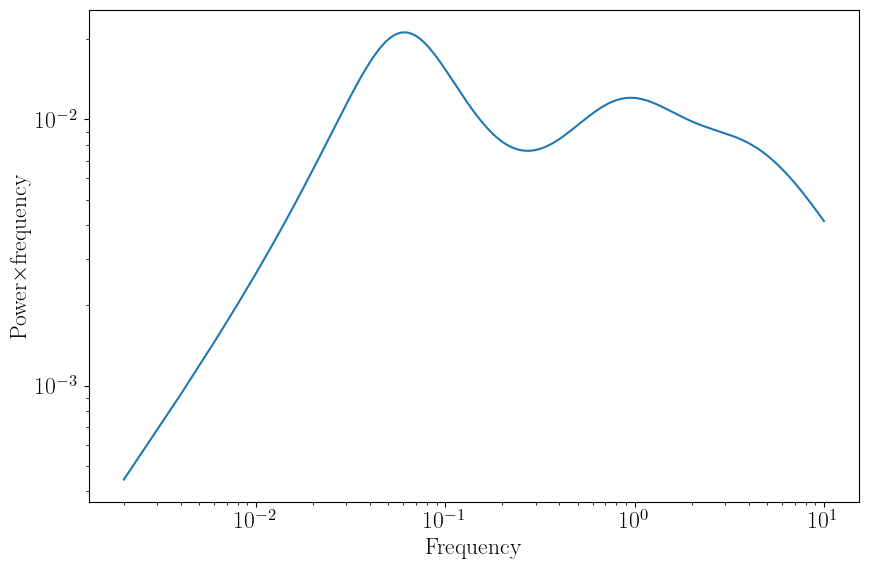
Having initialized our power spectrum object, we can decide what kind of model it will contain. For this simulation, we will use three Lorentzians to make up broadband noise similar to that observed in black hole X-ray binaries:

def lorentz(freq,peak_f,q,rms):
    par_array = np.array([peak_f,q,rms])
    model = models.lorentz(freq,par_array)
    return model

#Define our model for the power spectrum directly in Fourier space, as a sum of
#two Lorentzians
Lorentz_model = LM_Model(lorentz, prefix="l1_") + \
                LM_Model(lorentz, prefix="l2_") + \
                LM_Model(lorentz, prefix="l3_")

Lorentz_model_parameters = LM_Parameters()
Lorentz_model_parameters.add_many(('l1_peak_f', 0.06, True, 1e-3, 0.3),
                                  ('l1_q', 0.5, True, 0, 2),
                                  ('l1_rms', 0.20, True),
                                  ('l2_peak_f', 0.9, True, 0.3, 1.25),
                                  ('l2_q', 0.3, True, 0, 2),
                                  ('l2_rms', 0.15, True),
                                  ('l3_peak_f', 4.0, True, 1.25, 10),
                                  ('l3_q', 0.2, True, 0, 2),
                                  ('l3_rms', 0.12, True),
                                 )

#Assign the model array to power_spec and plot the result
psd_model.set_psd_model(Lorentz_model,Lorentz_model_parameters)
psd_model.compute_psd()
psd_model.plot_psd()
gc.collect()

15479

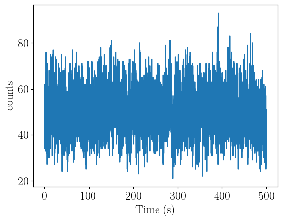
Once the observation details and model are specified, we can then assume some expected source count rate use the simulate_lightcurve function to create a stingray Lightcurve object, which contains the counts per bin over the simulated observation. As a sanity check, we can ensure that the mean count rate is indeed identical to our input:

from ndspec.Simulator import simulate_lightcurve

countrate = 1000

simulated_observation = simulate_lightcurve(psd_model,obs_time,dt,countrate)

simulated_observation.plot()

<Axes: xlabel='Time (s)', ylabel='counts'>

print(np.mean(simulated_observation.counts)/dt)

1000.198

How to simulate a time-averaged spectrum

Simulating a time-averaged spectrum is similar, but we also need to specify an instrument response matrix to be used in the simulation. In this case, we will use the FPMA detector on NuSTAR:

nustar = os.getcwd() + "/data/"

rmfpath = nustar + "/nu90401309004A01_sr.rmf"
fpma = ResponseMatrix(rmfpath)
arfpath = nustar + "/nu90401309004A01_sr.arf"
fpma.load_arf(arfpath)

Arf missing, please load it
Arf loaded

For our model we will use the Xspec model interface provided by nDspec. We will simulate a standard combination of accretion disk emission (diskbb) and coronal power-law emission (powerlaw), absorbed by neutral gas (tbabs). For the model parameters we will pick some sensible value resembling a hard state X-ray binary:

import ndspec.XspecInterface as xsmodels

def tbabs(ear, params):
    pass

def powerlaw(ear, params):
    pass

def diskbb(ear, params):
    pass

xspec_library = xsmodels.FortranInterface()

xspec_library.load_models({
    "tbabs": tbabs,
    "powerlaw": powerlaw,
    "diskbb": diskbb,
})

def ndspec_tbabs(ear,nH):
    par_array = np.array([nH])
    model = xspec_library.tbabs(ear,par_array)
    return model

def ndspec_powerlaw(ear,gamma,norm_pl):
    par_array = np.array([gamma,norm_pl])
    model = xspec_library.powerlaw(ear,par_array)
    return model

def ndspec_diskbb(ear,Tin,norm_dbb):
    norm_dbb = 10**norm_dbb
    par_array = np.array([Tin,norm_dbb])
    model = xspec_library.diskbb(ear,par_array)
    return model

sim_model = LM_Model(ndspec_tbabs)*(LM_Model(ndspec_diskbb)+LM_Model(ndspec_powerlaw))

#make sure that these normalizations make sense for xspec models as well
sim_params = sim_model.make_params(nH=dict(value=0.1,min=0.05,max=100,vary=True),
                                   Tin=dict(value=0.25,min=0.15,max=5.,vary=True),
                                   norm_dbb=dict(value=5.7,min=-2.,max=8.,vary=True),
                                   gamma=dict(value=1.6,min=1.3,max=3.5,vary=True),
                                   norm_pl=dict(value=6,min=1e-1,max=1e6,vary=True)
                                   )


xspec_library.print_model_info()

Initialized Xspec models:
tbabs:
  type: mul
  function called: C_tbabs
  parameters:
    nH: value: 1.0, min: 0.0, max: 1000000.0, unit: 10^22

powerlaw:
  type: add
  function called: C_powerLaw
  parameters:
    PhoIndex: value: 1.0, min: -3.0, max: 10.0, unit: n/a
    norm: value: 1, min: 0, max: 1e+20, unit: n/a

diskbb:
  type: add
  function called: xsdskb
  parameters:
    Tin: value: 1.0, min: 0.0, max: 1000.0, unit: keV
    norm: value: 1, min: 0, max: 1e+20, unit: n/a

 Solar Abundance Vector set to angr:  Anders E. & Grevesse N. Geochimica et Cosmochimica Acta 53, 197 (1989)
 Cross Section Table set to vern:  Verner, Ferland, Korista, and Yakovlev 1996

Once again, having defined the instrument response, model, model parameters, and observation time (in seconds), we can use the simulate_time_averaged function to create a Poisson realization of the assumed model, as observed through the detector we specified.

from ndspec.Simulator import simulate_time_averaged

exposure = 5e4

simulated_spectrum = simulate_time_averaged(fpma,sim_model,sim_params,exposure_time=exposure)

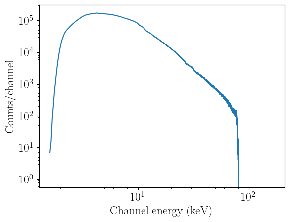
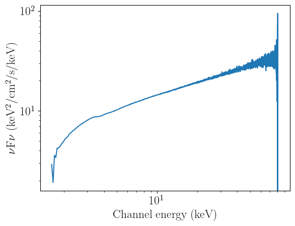
We can now plot the simulated_spectrum array, which is returned in units of counts/channel, as well as unfold it to retrieve the original model in units of physical flux (here, kev per unit time and area):

midpoint = 0.5*(fpma.emax+fpma.emin)

plt.figure(1)
plt.loglog(midpoint,simulated_spectrum)
plt.xlabel("Channel energy (keV)")
plt.ylabel("Counts/channel")

plt.figure(2)
plt.loglog(midpoint,fpma.unfold_response(simulated_spectrum,units_in="channel")*midpoint**2/5e4)
plt.xlabel("Channel energy (keV)")
plt.ylabel("$\\rm{\\nu}$F$\\rm{\\nu}$ (keV$^2$/cm$^2$/s/keV)")
gc.collect()

/home/matteo/Software/nDspec/src/ndspec/Response.py:653: RuntimeWarning: invalid value encountered in divide
  unfold_model = array/unfold_array

20

How to simulate a lag energy spectrum

Simulating a lag-energy spectrum is more complex, as it requires the user make more assumptions. First, we must set up an instrument response that has been binned to a sufficiently coarse number of channels of interest - here we will use 20 channels, spaced between 3 and 78 keV. The methodology described here is identical to that of Ingram et al. 2022 (section 3), which we encourage users to read.

#turn the stuff above into a function
#first set up the response we want
rebin_grid = np.geomspace(3,78,21)
#include one channel between the start of the fpma response and 3keV, and one between 78 keV and the end of the response
rebin_grid = np.append(rebin_grid,fpma.emin[0])
rebin_grid = np.append(rebin_grid,fpma.emax[-1])
rebin_grid = np.unique(np.sort(rebin_grid))
rebin_fpma = fpma.rebin_channels(rebin_grid[:-1],rebin_grid[1:])

Having defined the instrument response we will use, we must make two more assumptions on the time-averaged spectrum of the source, as well as the instrument background, as both are needed to calculate the error bars for the lags. Here we will re-use the time-averaged spectrum from earlier, and very optimistically assume the background to be 0

#from the response, we take the energy grid and calculate the models
energ_grid = 0.5*(rebin_fpma.energ_lo+rebin_fpma.energ_hi)

#now we prepare the grid of energy bounds to calculate our spectral model, and calculate it
rebin_ear = np.append(rebin_fpma.energ_lo,rebin_fpma.energ_hi[-1])
spectrum_model = sim_model.eval(sim_params,ear=rebin_ear)

#next we set up the background - optimi
bkg_rate = np.zeros(rebin_fpma.n_chans-1)

Finally, we must build our model for the full cross spectrum, including both real and imaginary parts, as these are also required in the uncertainty calculation.

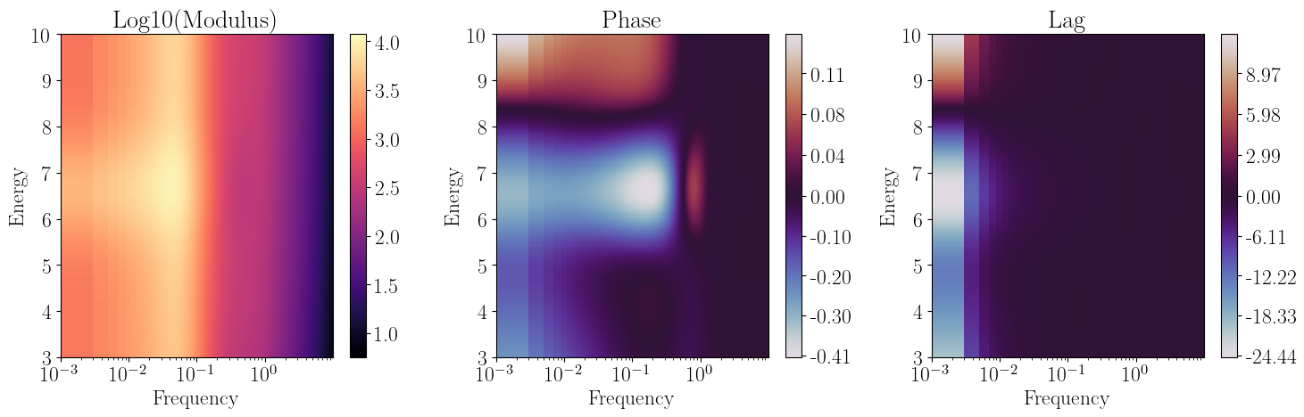
Here we will use a combination of (variable) corona emission, in the form of a pivoting power-law, and reverberation in the form of a Gaussian flash at 6.4 keV. The model parameters are similar as in the rest of the tutorials, except for the normalizations which have been adjusted to produce an absolute rms typical of a hard state X-ray binary:

#define the reference band to use - we will take the full NuSTAR band here
ref_emin = 3
ref_emax = 78

#first the pivoting powerlaw
pl_norm = 5.
pl_slope = -1.6
gamma_0 = 0.3
gamma_nu = -0.1
phi_0 = -0.3
phi_nu = -0.1
nu_0 = psd_model.freqs[0]
piv_transfer = models.pivoting_pl(psd_model.freqs,energ_grid,np.array([pl_norm,pl_slope,gamma_0,gamma_nu,phi_0,phi_nu,nu_0]))

continuum = CrossSpectrum(psd_model.times,energ=energ_grid)
continuum.set_transfer(piv_transfer)
continuum.set_psd_weights(psd_model.power_spec)
continuum.set_reference_energ([ref_emin,ref_emax])
continuum.cross_from_transfer()

#now the reverberation
gauss_norm = 2.5
gauss_sigma = 1.5
gauss_center = 6.5
rise_slope = 3
decay_slope = -2
peak_time = 15
width_slope = -0.2

gauss_flash = models.gauss_bkn(psd_model.times,energ_grid,
                               np.array([gauss_norm,gauss_sigma,gauss_center,rise_slope,
                                         decay_slope,peak_time,width_slope]),
                               )

reverb = CrossSpectrum(psd_model.times,energ=energ_grid)
reverb.set_psd_weights(psd_model.power_spec)
reverb.set_impulse(gauss_flash)
reverb.set_reference_energ([ref_emin,ref_emax])
reverb.cross_from_irf()

#finally we combine both
full_model = CrossSpectrum(psd_model.times,energ=energ_grid)
full_model.set_psd_weights(psd_model.power_spec)
full_model.set_transfer(continuum.trans_func + reverb.trans_func)
full_model.set_reference_energ([ref_emin,ref_emax])
full_model.cross_from_transfer()
full_model.plot_cross_2d(energy_limits=[3,10])
gc.collect()
#we are now ready to simulate our observation

67320

Having defined all of our models, all that remains is to specify the interval of Fourier frequency over which to simulate the lag spectrum, the coherence over these frequencies, the power (in units of fractional rms), and the assumed exposure time.

Once these are set,we can call the simulate_lag_energy function to re-derive our simulated lags

from ndspec.Simulator import simulate_lag_energy

fmin = 5e-3
fmax = 5e-2
coherence = 1
power = 5e-3
exposure = 5e4

lag_sim, lag_err, emin , emax = simulate_lag_energy(rebin_fpma,spectrum_model,full_model,
                                                    bkg_rate,[fmin,fmax],[ref_emin,ref_emax],
                                                    coherence,power,exposure)

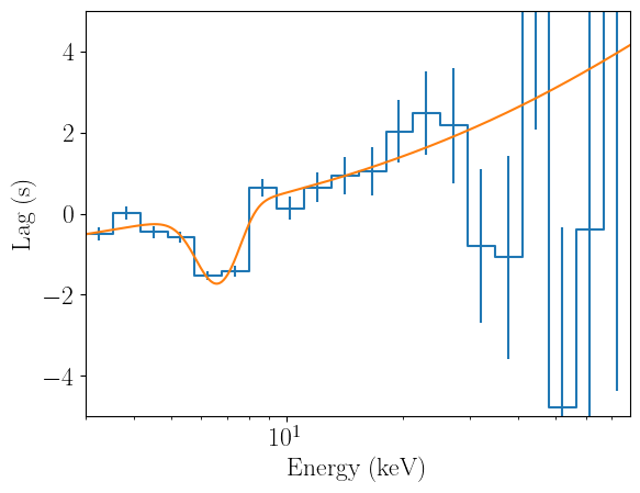
Finally, we can compare our simulated data with the original input model to reassure ourselves that the output makes sense:

ebounds = 0.5*(emin+emax)

plt.figure(1)
plt.step(ebounds,lag_sim,where='mid',color="C0")
plt.errorbar(ebounds,lag_sim,yerr=lag_err,ls="",color="C0")
plt.plot(full_model.energ,full_model.lag_energy([fmin,fmax]),color="C1")
plt.xscale("log",base=10)
plt.xlabel("Energy (keV)")
plt.ylabel("Lag (s)")
plt.ylim([-5,5])
plt.xlim([3,78])

(3, 78)